Motivic Cell Structure of Toric Surfaces

In this post I'll do a few very explicit computations for motivic cell structures of smooth projective toric varieties coming from the Białynicki-Birula decomposition, namely $\mathbb{P}^1, \mathbb{P}^1 \times \mathbb{P}^1, \mathbb{P}^2$ and Hirzebruch surfaces. It is a bit lengthy but maybe helpful to anyone who wants to do some explicit calculations with BB-decompositions. I hope you're accustomed to toric varieties, but I won't do anything fancy. You can safely skip the motivic part of this post.

I wrote about motivic cell structures and the Białynicki-Birula decomposition before. Here I'll explain how to compute a motivic cell structure out of the BB-decomposition explicitly and how to get an explicit BB-decomposition for any smooth complete toric variety. Then I'll do the examples.

Explicit Motivic Cell Structure

As described in the last post about Białynicki-Birula's Annals paper from 1972/73, for a $\mathbb{G}_m$-action on a smooth complete variety $X$ over a (possibly non-closed) field $k$ (of arbitrary characteristics), there is the plus-decomposition, giving us for each fixed point $a \in X^{\mathbb{G}_m}$ a subscheme $X_a^+ \subset X$ which is isomorphic to an affine space $X_a^+ \simeq \mathbb{A}^{n_a}$. The number $n_a$ is the dimension of the positive weight part (with respect to the induced $\mathbb{G}_m$-action) of the (co)tangent space of $X$ at $a$.

There is another paper of Białynicki-Birula, published in 1976 in the Bulletin de l'académie polonaise des sciences, Série des sciences math., where it is proved that the BB-decomposition of smooth projective varieties is filtrable, which means that one can choose an order on the fixed points $X^{\mathbb{G}_m} = \{a_0,\dots,a_m\}$ and a partition of $m$ into $d$ blocks (where $d$ is the dimension of $X$) such that for $X_i$ the union of cells of each block, the $X_i$ are closed subschemes of $X$ that form a finite decreasing sequence
$! X = X_d \supset X_{d-1} \supset \cdots \supset X_{0} \supset X_{-1} = \emptyset.$ Here every $\supset$ is a proper inclusion. The proof uses Sumihiro's equivariant completion, which provides an equivariant closed immersion into a projective space with linear torus action, so there one can filter the projective space by the weights of this action and that provides the closed immersions. If one wants to compute something, one can of course figure out a good order of the fixed points by hand, without looking at equivariant embeddings at all. At the moment, I don't know any algorithm other than brute force to do that.

Now we build a motivic cell structure out of this. This is slightly unusual, as the attaching maps arise "the other way around" than one would expect. If it confuses you, the examples below might provide illumination.
The open subscheme $X \setminus X_i \to X \setminus X_{i-1}$ has complement isomorphic to a disjoint union of some $X^+_{a_i}$.
Look at the closed immersion of smooth schemes $\iota : X_{a_i}^+ \to X \setminus X_{i-1}$ and its normal bundle $N_{\iota}$. By the homotopy purity theorem of Morel and Voevodsky we have
$! N_\iota / (N_\iota \setminus X^+_{a_i}) =: Th(N_{\iota}) \simeq (X \setminus X_{i-1}) / ((X \setminus X_{i-1})\setminus \iota(X_{a_i}^+)$ $! = (X \setminus X_{i-1}) / (X \setminus X_i) \simeq S^{2n_i,n_i}.$ If we want to handle more cells at once, we just define $Th(N_i)$ by
$X \setminus X_i \to X \setminus X_{i-1} \to Th(N_i)$
to be a homotopy cofiber sequence.
One more homotopy cofiber construction gives us $Th(N_i) \to \Sigma (X \setminus X_i)$, an attaching map of $Th(N_i) \sim \bigvee S^{2n_\alpha,n_\alpha}$ into $\Sigma (X \setminus X_i)$ that gives us, as next homotopy cofiber, the space $\Sigma (X \setminus X_{i-1})$. So this produces inductively a stable motivic cell structure on $X$, since for $A \to B \to C$ a cofiber sequence with two stably cellular spaces, a theorem of Dugger and Isaksen shows that the third space is also stably cellular.

That toric varieties have a motivic cell structure (without referring to the BB-decomposition) is already contained in the paper of Dugger and Isaksen Motivic Cell Structures.

Motives

From a homotopy cofiber sequence $X \to Y \to Z \to \cdots$ we get a distinguished triangle in the category of motives $DM_-$ of the reduced motives $\tilde{h}(X) \to \tilde{h}(Y) \to \tilde{h}(Z) \to[1] \cdots$. Like with reduced and unreduces cohomology theories, $\tilde{h}(Y) \oplus \mathbb{Z} = h(Y)$, so we can compute motives of varieties from homotopy cofiber sequences.

Concrete $\mathbb{G}_m$-actions with isolated fixed points

It is long known for toric varieties, that any torus cocharacter in general position (in the cocharacter lattice) has the same fixed points as the torus. To describe explicit cell decompositions, one needs to know which cocharacter is "in general position" and which cocharacter has a larger fixed point set. A cocharacter $\alpha$ fixes an orbit $O_\tau$ if $\alpha$ is inside the linear subspace generated by $\tau$. The full torus has as fixed points those $O_\tau$ with $\tau$ of maximal dimension. To pick a good cocharacter, one just has to avoid the hyperplanes spanned by the codimension 1 cones in the fan.

The Projective Line

The fan of the projective line consists of the cone $\{0\}$ and the cones generated by $1$ and $-1$ respectively. The affine variety corresponding to the $1$-cone is $\mathbb{A}^1_0 := \mathbb{P}^1 \setminus \{\infty\} \subset \mathbb{P}^1$ and the affine variety corresponding to the $-1$-cone is $\mathbb{A}^1_\infty := \mathbb{P}^1 \setminus \{0\} \subset \mathbb{P}^1$. Their intersection is the affine variety corresponding to the cone $\{0\}$, which is the torus $\mathbb{G}_m = \mathbb{P}^1 \setminus \{0,\infty\}$.

The torus $\mathbb{G}_m$ acts on itself via the group multiplication, and it acts on $\{0\}$ and $\{\infty\}$ trivially, i.e. these are the fixed points of the action. If you prefer homogeneous coordinates, $\lambda \in \mathbb{G}_m(k)$ acts on $[x:y] \in \mathbb{P}^1(k)$ as $\lambda.[x:y] = [\lambda x : y]$, so we have $\lambda.[0:1] = [0:1]$ and $\lambda.[1:0] = [\lambda:0] = [1:0]$.

The Kähler differentials are $\Omega^1_{\mathbb{P}^1/k,0} \simeq \Omega^1_{\mathbb{A}^1_0/k,0} = \langle dX \rangle_k$ and $\Omega^1_{\mathbb{P}^1/k,\infty} \simeq \Omega^1_{\mathbb{A}^1_\infty/k,0} = \langle dX^{-1} \rangle_k$. The induced $\mathbb{G}_m(k)$-action is $\lambda.dX = \lambda dX$ and $\lambda.dX^{-1} = \lambda^{-1} dX^{-1}$, respectively. We see that the positive weight part at $0$ is everything, while at $\infty$ it is nothing. Consequently, the orthogonal at $0$ is nothing and at $\infty$ it is everything. Under $\mathfrak{m} \to \mathfrak{m}/\mathfrak{m}^2$ we get an isomorphic preimage of this orthogonal and take the ideal generated by it. This gives us ideals $\mathfrak{n}_0 = (0)$ and $\mathfrak{n}_\infty = (X^{-1})$. They correspond to the cells $X_0^+ = V(\mathfrak{n}_0) = \mathbb{A}^1_0$ and $X_\infty^+ = V(\mathfrak{n}_\infty) = \{\infty\}$.

This is already the BB-decomposition: $\mathbb{P}^1 = \mathbb{A}^1 \cup \{\infty\}$.
The BB-filtration $X = X_d \supset X_{d-1} \supset \cdots \supset X_{0} \supset X_{-1} = \emptyset.$ of $X = \mathbb{P}^1$ is (with $d=1$) just $\mathbb{P}^1 \supset \{\infty\}$.
To get a motivic cell structure, we need attaching maps for the cell $Th(N_\iota) \simeq X/X_0 = \mathbb{P}^1 \simeq S^{2,1}$ to the set of $0$-cells $X_0 = \{\infty\}$. The stable attaching map is the cofibration $S^{2,1} \to \Sigma (\mathbb{P}^1 \setminus \{\infty\})$, which one can see as the homotopy cofiber of $\mathbb{P}^1 \to \mathbb{P}^1$, i.e. the gluing of $\mathbb{P}^1$ along $\infty$ to a point $\infty$.

The homotopy cofiber sequence yields a distinguished triangle
$! \tilde{h}(\mathbb{P}^1) \to \tilde{h}(S^{2,1}) \to \tilde{h}(\Sigma (\mathbb{P}^1 \setminus \{\infty\})) \to \tilde{h}(\mathbb{P}^1)[1] \to \cdots$ which we can identify as
$! \tilde{h}(\mathbb{P}^1) \to \mathbb{Z}(1)[2] \to 0 \to \cdots.$ Now we have a splitting $\tilde{h}(\mathbb{P}^1) = \mathbb{Z}(1)[2]$.

Okay, that was kind of stupid, given that we already knew that $\mathbb{P}^1$ is a $(2,1)$-cell. It was also kind of stupid that we have computed a stable cell structure, while it is also quite easy to describe an unstable cell structure of projective spaces.

We can also take a different $\mathbb{G}_m$-action on $\mathbb{P}^1$, by taking any cocharacter (i.e. group homomorphism) $\mathbb{G}_m \to \mathbb{G}_m$. These are all of the form $\lambda \mapsto \lambda^n$ for some $n \in \mathbb{Z}$. If $n > 0$, we get the same weight decomposition of (co)tangent spaces (Kähler differentials), hence the same BB-decomposition. If $n = 0$, we get no decomposition because the fixed points are not isolated (they are everything). If $n < 0$, we get the decomposition $\mathbb{P}^1 = \{0\} \cup \mathbb{A}^1_\infty$, which one might also call the minus-decomposition w.r.t. the first action considered.

A product of two lines

Here we have a torus $\mathbb{G}_m \times \mathbb{G}_m$ acting and it becomes a slightly more interesting question which cocharacter $\mathbb{G}_m \to \mathbb{G}_m \times \mathbb{G}_m$ gives which BB-decomposition.

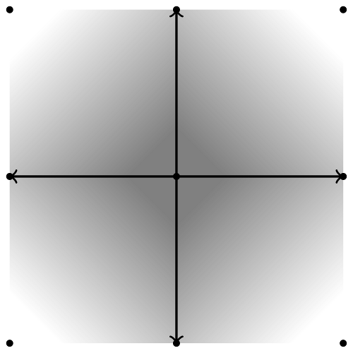
The fixed points of the torus are the orbit closures corresponding to the maximal cones, which are $(0,0),(0,\infty),(\infty,\infty),(\infty,0)$.

Take the diagonal $\lambda \mapsto (\lambda,\lambda)$ corresponding to the weight $(1,1)$ in the weight lattice. It doesn't hit any linear subspace generated by codimension one cones, so it has the same isolated fixed points, as the original torus. (In contrast, e.g. $\lambda \mapsto (\lambda,1)$ fixes a whole $\{0\} \times \mathbb{P}^1$).

From analyzing the positive weight subspaces of the cotangent spaces of $\mathbb{P}^1 \times \mathbb{P}^1$ at these fixed points, we get
$(\Omega^1_{(0,0)})^+ = \langle dX,dY\rangle_k$
$(\Omega^1_{(0,\infty)})^+ = \langle dX\rangle_k$
$(\Omega^1_{(\infty,\infty)})^+ = 0$
$(\Omega^1_{(\infty,0)})^+ = \langle dY\rangle_k$
and from this the ideals defining the cells
$\mathfrak{n}_{(0,0)} = (0) \leq k[X,Y]$
$\mathfrak{n}_{(0,\infty)} = (Y^{-1}) \leq k[X,Y^{-1}]$
$\mathfrak{n}_{(\infty,\infty)} = (X^{-1},Y^{-1}) \leq k[X^{-1},Y^{-1}]$
$\mathfrak{n}_{(\infty,0)} = (X^{-1}) \leq k[X^{-1},Y]$
so the cells are
$X^+_{(0,0)} = \mathbb{A}^1_0 \times \mathbb{A}^1_0$
$X^+_{(0,\infty)} = \mathbb{A}^1_0 \times \{\infty\}$
$X^+_{(\infty,\infty)} = \{(\infty,\infty)\}$
$X^+_{(\infty,0)} = \{\infty\} \times \mathbb{A}^1_0$

It is pretty obvious now how much influence the choice of a cocharacter has on the cell decomposition. There are only four different cell decompositions, corresponding to the four maximal-dimensional cones in the fan.

The BB-filtration is $\mathbb{P}^1 \times \mathbb{P}^1 \supset \mathbb{P}^1 \times \{\infty\} \cup \{\infty\} \times \mathbb{P}^1 \supset \{(\infty,\infty)\} \supset \emptyset$. The motivic cell structure is built inductively, we start with the cellular space $\{(\infty,\infty)\} \simeq \mathbb{A}^1 \times \mathbb{A}^1$ and attach the cellular space $Th(N_1) \simeq S^{2,1} \vee S^{2,1}$ to it (to obtain $\mathbb{P}^1\times\mathbb{P}^1 \setminus \{(\infty,\infty)\}$) via the homotopy cofiber sequence
$! \mathbb{A}^1 \times \mathbb{A}^1 \to \mathbb{P}^1\times\mathbb{P}^1 \setminus \{(\infty,\infty)\} \to Th(N_1) \to \Sigma (\mathbb{A}^1 \times \mathbb{A}^1).$ In the next step we attach to the stably cellular space $\mathbb{P}^1\times\mathbb{P}^1 \setminus \{(\infty,\infty)\}$ the cellular space $Th(N_0) \simeq S^{4,2}$ to obtain $\mathbb{P}^1 \times \mathbb{P}^1$ via the homotopy cofiber sequence
$! \mathbb{P}^1\times\mathbb{P}^1 \setminus \{(\infty,\infty)\} \to \mathbb{P}^1 \times \mathbb{P}^1 \to Th(N_0) \to \Sigma(\mathbb{P}^1\times\mathbb{P}^1 \setminus \{(\infty,\infty)\}).$

This is also the motivic cell structure you would get as product cell structure from the previously considered cell structure for $\mathbb{P}^1$, and it is all parallel to classical topology, up to homotopy (though classically the gluing maps don't look that strange).

For the sake of completeness, let's compute the motive from this (i.e. let's look at the distinguished triangles):
$! 0 \to \tilde{h}(\mathbb{P}^1\times\mathbb{P}^1 \setminus \{(\infty,\infty)\})) \to \mathbb{Z}(1)[2] \oplus \mathbb{Z}(1)[2] \to 0 \to \cdots$ shows that $\tilde{h}(\mathbb{P}^1\times\mathbb{P}^1 \setminus \{(\infty,\infty)\})) = \mathbb{Z}(1)[2] \oplus \mathbb{Z}(1)[2]$, as expected from the observation $\mathbb{P}^1\times\mathbb{P}^1 \setminus \{(\infty,\infty)\}) \simeq \mathbb{P}^1 \vee \mathbb{P}^1 \simeq S^{2,1} \vee S^{2,1}$. The next homotopy cofiber sequence gives
$! \mathbb{Z}(1)[2] \oplus \mathbb{Z}(1)[2] \to \tilde{h}(\mathbb{P}^1 \times \mathbb{P}^1) \to \mathbb{Z}(2)[4] \to \mathbb{Z}(1)[3] \oplus \mathbb{Z}(1)[3] \to \cdots$ and we get $\tilde{h}(\mathbb{P}^1 \times \mathbb{P}^1) = \mathbb{Z}(1)[2] \oplus \mathbb{Z}(1)[2] \oplus \mathbb{Z}(2)[4]$, since there are no non-trivial morphisms $\mathbb{Z}(2)[4] \to \mathbb{Z}(1)[3]$.

The Projective Plane

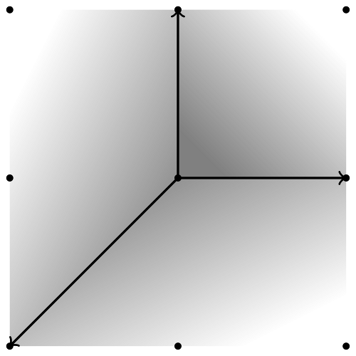
The fixed points of the torus $\mathbb{G}_m \times \mathbb{G}_m$ are $[0:0:1]$, $[1:0:0]$ and $[0:1:0]$ (corresponding to the maximal dimensional cones $1,2,3$ in the fan, in counter-clockwise order). Denote by $U_i$ the affine toric variety corresponding to the maximal dimensional cone $i$.

The cotangent spaces at the fixed points are
$\Omega_{\mathbb{P}^2,[0:0:1]} = \Omega_{U_1,(0,0)} = \langle dX, dY \rangle_k$,
$\Omega_{\mathbb{P}^2,[1:0:0]} = \Omega_{U_2,(0,0)} = \langle dX^{-1}Y, dX^{-1} \rangle_k$,
$\Omega_{\mathbb{P}^2,[0:1:0]} = \Omega_{U_3,(0,0)} = \langle dXY^{-1}, dY^{-1} \rangle_k$.

The diagonal cocharacter $\lambda \mapsto (\lambda,\lambda)$ is no longer good, since $(1,1)$ lies in the linear subspace generated by a cone of the fan -- it fixes the projective line $\{[x:y:0] | [x:y] \in \mathbb{P}^1\}$.

We can choose the cocharacter $\lambda \mapsto (\lambda^{-1},\lambda)$, which acts with the same isolated fixed points as the whole torus on $\mathbb{P}^2$. For this one we get:
$(\Omega^1_{[0:0:1]})^+ = \langle dY \rangle_k$,
$(\Omega^1_{[1:0:0]})^+ = \langle dX^{-1}Y, dX^{-1} \rangle_k$,
$(\Omega^1_{[0:1:0]})^+ = 0$,
so that we have cells
$X^+_{[0:0:1]} = V(X) = \{[0:y:1] | y \in \mathbb{A}^1\} \subset U_1$,
$X^+_{[1:0:0]} = V(0) = U_2 \simeq \mathbb{A}^2$,
$X^+_{[0:1:0]} = \{[0:1:0]\}$.
This decomposition is one of the common decompositions of $\mathbb{P}^2$ into $\mathbb{A}^2$ and a $\mathbb{P}^1$ at infinity, which is decomposed into $\mathbb{A}^1$ and $\infty$.
The corresponding BB-filtration is just $\mathbb{P}^2 \supset \mathbb{P}^1 \supset \mathbb{P}^0$.

The homotopy cofiber sequences that give the motivic cell structure are
$! \mathbb{A}^2 \to \mathbb{P}^2 \setminus \mathbb{P}^0 \to Th(N_1) \simeq S^{2,1} \to \Sigma \mathbb{A}^2$
$! \mathbb{P}^2 \setminus \mathbb{P}^0 \to \mathbb{P}^2 \to Th(N_0) \simeq S^{4,2} \to \Sigma(\mathbb{P}^2 \setminus \mathbb{P}^0).$
As before, we have $\tilde{h}(\mathbb{P}^2 \setminus \mathbb{P}^0) = \mathbb{Z}(1)[2]$ and $\tilde{h}(\mathbb{P}^2) = \mathbb{Z}(1)[2] \oplus \mathbb{Z}(2)[4]$.

If we pick another cocharacter $\lambda \mapsto (\lambda^{-2},\lambda^{-1})$, this is still inside the cone $2$, but it has a different scalar product with one of the rays, so the decomposition should be different. Indeed, from computations we find that the big cell now is part of $U_3$ and in $U_2$ we have only a $0$-cell.

Hirzebruch surfaces

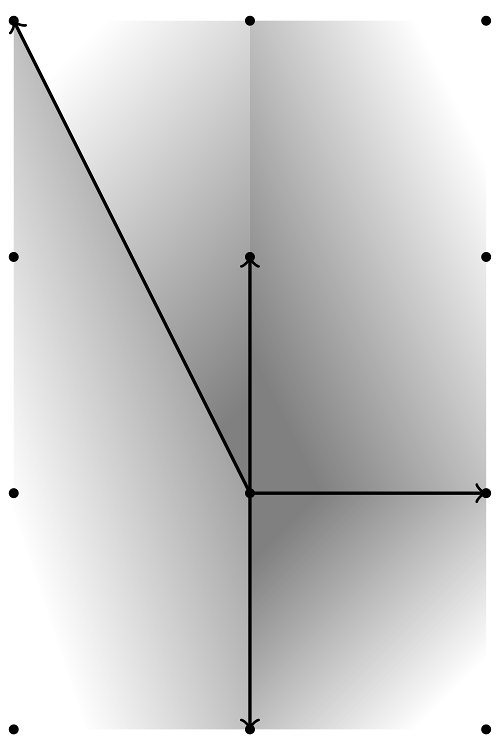
The fan for a Hirzebruch surface $\mathbb{F}_a = \mathbb{P}(\mathcal{O}(a) \oplus \mathcal{O})$ looks similar to the fan of $\mathbb{P}^1\times\mathbb{P}^1 = \mathbb{P}(\mathcal{O} \oplus \mathcal{O})$:

The image shows the fan of $\mathbb{F}_2$.

We pick the torus cocharacter of weight $(1,1)$ again, since it works for all Hirzebruch surfaces.

The cone generated by $(0,1)$ and $(1,0)$ as well as the cone generated by $(1,0)$ and $(0,-1)$ are just as in the situation of $\mathbb{F}_0 = \mathbb{P}^1 \times \mathbb{P}^1$, and the corresponding affine toric varieties glue together to a $\mathbb{P}^1 \times \mathbb{A}^1$, which is visible in the cell structure. The big cell is $\mathbb{A}^2$ corresponding to the cone with faces $(0,1)$ and $(1,0)$.

The cone generated by $(-1,a)$ and $(0,-1)$ corresponds to a fixed point which is a BB-cell itself and the cone generated by $(0,1)$ and $(-1,a)$ corresponds to a fixed point with attached BB-cell of dimension $1$.

The BB-filtration is $\mathbb{F}_a = X_2 \supset X_1 \supset X_0 \supset \emptyset$ with $X_0$ the fixed point which already is a cell and $X_1$ everything except the big cell (big cell = unique open cell). The motivic cell structure is built from the homotopy cofiber sequences
$! \mathbb{A}^2 \to \mathbb{F}_a \setminus X_0 \to Th(N_1) \to \Sigma \mathbb{A}^2$
$! \mathbb{F}_a \setminus X_0 \to \mathbb{F}_a \to Th(N_0) \to \Sigma(\mathbb{F}_a \setminus X_0).$
The space $\mathbb{F}_a \setminus X_0$ is homotopy equivalent to the $\mathbb{P}^1$ at the base, but the gluing map $Th(N_0) \to \Sigma(\mathbb{F}_a \setminus X_0)$ really depends on $a$.

The motive is just the same as the motive of $\mathbb{P}^1 \times \mathbb{P}^1$.

More complete nonsingular surfaces

It is a well-known fact (and not hard to prove) that all complete nonsingular toric surfaces (implicitly assuming normal) are either $\mathbb{P}^2$, a Hirzebruch surface $\mathbb{F}_a$ or a blow-up of one of these at torus fixed points, since one can describe such blow-ups with fans. One easily sees that blowing up a fixed point introduces an additional fixed point with "BB-cell" $\mathbb{A}^1$, therefore an additional $S^{2,1}$ to the motivic cell structure (the additional $\mathbb{P}^1$). This introduces an additional $\mathbb{Z}(1)[2]$ to the motive.